• Home   
• About   
• Blog   

Creating Realistic Terrain by Modelling the Physics of Hydraulic Erosion

November 2025 (5574 Words, 31 Minutes)

In this post, we’ll explore how to significantly enhance procedurally generated terrain using hydraulic erosion. By simulating the natural processes that shape real-world landscapes, we can transform basic noise-generated height maps into believable terrains that exhibit realistic features like river valleys, sediment deposits, and asymmetric slopes.

Here’s a sneak peak at what we’ll be getting into and the kind of results you can achieve:

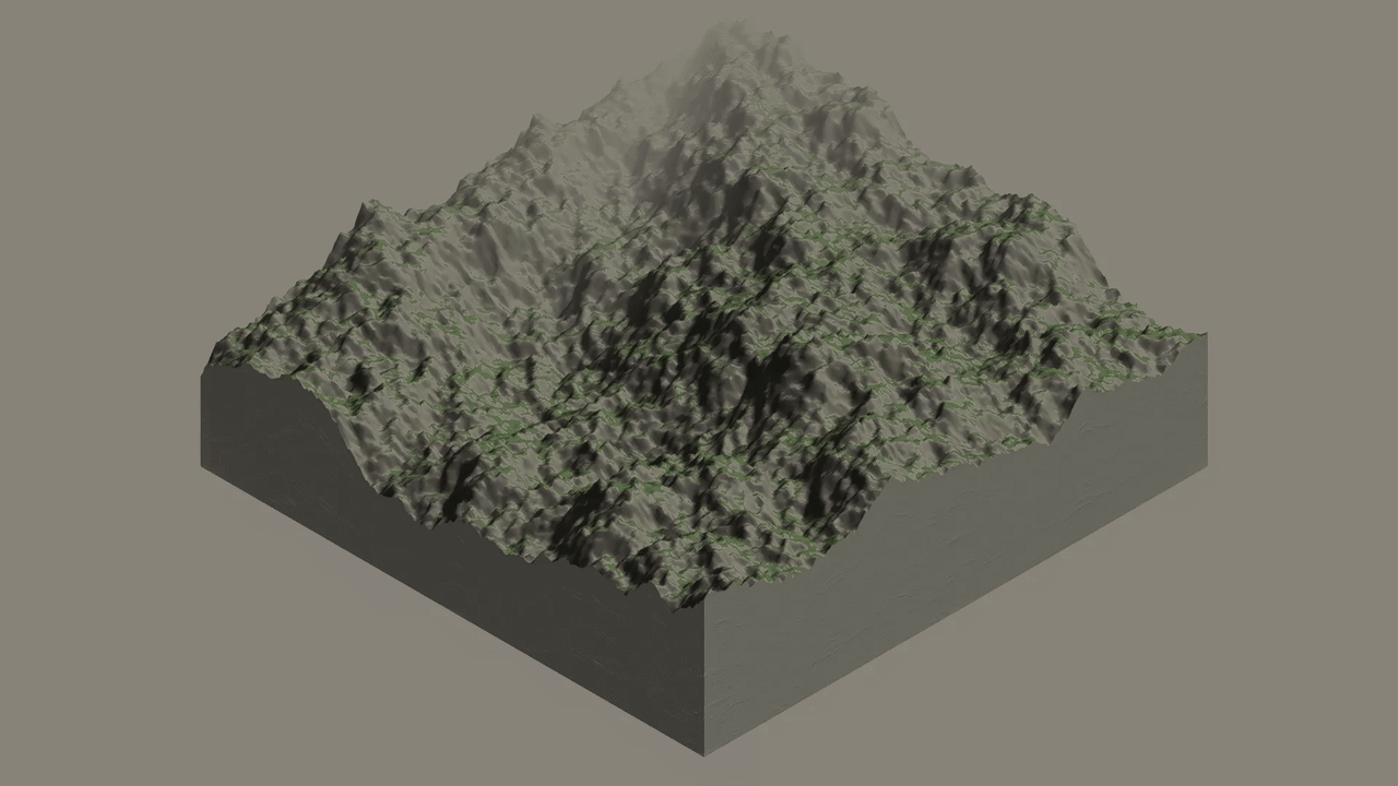
Table of Contents

• The Problem: Noise
• The Solution: Hydraulic Erosion
  • Research and References
• Modelling Erosion
• Sneak Peek!
  • Theory
  • Understanding the Terrain Grid
  • Implementation
• What’s Next?
• References

The Problem: Noise

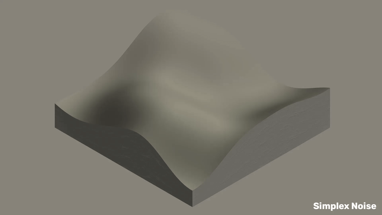
Procedural generation is everywhere in games and simulations from sprawling open-world RPGs to flight simulators to rogue-lite games where you’ll never play the same level twice. When generating terrain procedurally, most algorithms rely on noise functions like Perlin Noise, or its successor Simplex Noise. Below you can see examples of terrain generated using the Simplex noise function, with smooth and continuous rolling hills thanks to its spatially coherent nature:

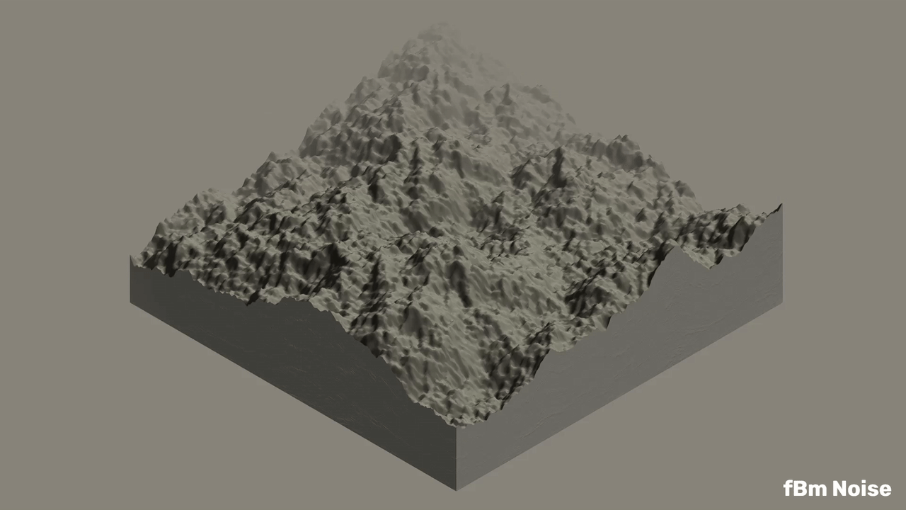
We can introduce some complexity and detail using techniques like Fractional Brownian Motion (fBm) that layer multiple octaves of noise, or Ridged Noise to create sharper peaks. Here are some examples of terrains generated using fBm:

But you may have noticed that they all share a subtle problem: the mountains are too uniform, the valleys too smooth, the whole thing too… mathematical.

Terrain generated using these noise functions can very easily fall into the Uncanny Valley where they look almost right, but to the human eye something looks off. What we’re missing are the core characteristic features of real terrain: carved river valleys, natural drainage patterns, sediment deposits, and the asymmetric character that comes from millenia of Mother Nature working her magic.

The Solution: Hydraulic Erosion

So what if we tried to simulate these forces of nature? What if we took our procedurally generated rolling hills, and simulated the effects of rainfall and water flowing across them? That is the essence of hydraulic erosion!

Hydraulic erosion is a simulation technique that models how water shapes terrain over time. In the real world, rainfall and flowing water are the primary sculptors of landscapes.

The basic principle is elegant: water falls on terrain, flows downhill following gravity, picks up sediment where it flows fast (erosion), and deposits sediment where it slows down (deposition). Repeat this process millions of times, and you get realistic-looking terrain features that emerge naturally based on physics.

Erosion is typically applied as a post-processing step after generating a base height map using noise functions, and can be implemented to run offline or in real-time.

Research and References

Hydraulic erosion has been studied extensively in computer graphics research. The foundational work by Musgrave et al.¹ back in 1989 introduced physical erosion models to terrain generation. Modern approaches fall into two main categories:

• Particle-based: simulates individual water droplets following Newtonian mechanics.^{2 3 4}
• Grid-based: simulates water flow using shallow water equations.^{5 6}

Both approaches can produce realistic results, with particle methods offering more flexibility and grid methods potentially running faster when implemented on the GPU. In this post, we’ll focus on a particle-based approach with an elegant physics-based mechanism.

Modelling Erosion

In our particle-based simulation, we simulate individual water droplets flowing across the terrain with the following simplified algorithm:

1. Spawn a droplet at a random position on the terrain.
2. Move the droplet downhill, following the terrain’s slope.
3. Calculate how much sediment the water can carry based on its speed and volume.
4. Erode terrain where water flows fast, OR Deposit sediment where it slows down.
5. Evaporate water gradually until the droplet disappears.
6. Repeat for thousands or millions of droplets!

The magic happens in aggregate — as each droplet independently follows a path based on its individual physical properties, they collectively carve organic-looking river networks and drainage patterns. These features emerge by themselves, without any explicit programming. Where one droplet carves a valley, others naturally follow the same path, deepening it over time.

Sneak Peek!

We’re about to dive into some heavy math and code, so before we do, here are a few before and after shots to help motivate you through to the end:

The results are striking! Here, I’ve applied a simple shader to give it a bit more character and show off the distinct erosion patterns. You can really see how we’re able to carve out realistic river valleys, deposit sediment in floodplains, and sculpt asymmetric slopes that feel organic rather than algorithmic.

Theory

The most straightforward and physically accurate approach uses classical mechanics equations to model water droplet behavior. In doing so, we can produce fantastically natural-looking results with minimal tuning. Droplets are tracked with four key state variables that are updated as they move:

• Position: where it is on the terrain (updated by velocity)
• Velocity: how fast and in what direction it’s moving (influenced by terrain slope and friction)
• Water volume: the total volume of water (decreases through evaporation)
• Sediment load: the percentage of water volume that is sediment (changes through erosion and deposition)

At each time step Δt, we update the droplet’s state using the following equations:

1. Force and Acceleration

The droplet accelerates due to gravity projected onto the terrain surface, forcing the droplet downhill.

Newton’s second law gives us:

where the mass m is the product of density ρ and water volume V_water:

The acceleration is derived from the surface normal vector n, which encodes the slope:

where n_xz represents the x and z components of the surface normal (the horizontal components).

2. Velocity Update

Using forward Euler integration, we update the velocity v based on the above acceleration and delta time:

We then apply friction to eventually slow the droplet down, which reduces velocity proportionally:

where μ is the friction coefficient.

3. Position Update

The droplet’s position is integrated using its velocity:

4. Sediment Capacity

The droplet’s sediment capacity (maximum amount of sediment it can carry) is recalculated at each step based on its current water volume, speed, and the terrain slope:

where C is the sediment capacity, the speed is defined as:

and the height difference is:

With higher water volume, speed and steeper slopes, the sediment capacity increases. When the droplet starts heading uphill (even by a small amount) or slowing down, capacity will decrease and the droplet will begin depositing sediment.

5. Erosion/Deposition

When the droplet is carrying less sediment than its capacity allows (C > s), it erodes the terrain. When it’s carrying more than it can handle (C < s), it deposits sediment. The sediment updates as follows:

where K_d is the deposition rate constant.

The terrain height is updated correspondingly at the droplet’s current cell:

The great thing about this approach is that we don’t need to include any special forking behavior for erosion vs. deposition in our code.

6. Evaporation

Water evaporates at a constant rate:

where K_e is the evaporation rate constant. The simulation ends when the water volume drops below a minimum threshold:

This simple mechanism, repeated millions of times, creates realistic erosion patterns.

Understanding the Terrain Grid

Before diving into the implementation, it’s important to understand how the terrain is represented and how droplets interact with it.

Discrete Grid Representation

The terrain heightmap is conceptually a discrete 2D grid of height values, where each cell represents a square region of the terrain surface. Think of it like a chessboard where each square has an associated height value.

Each cell (x, y) stores a single height value. The heightmap is stored as a 1D array, so the index is calculated as:

In this example, h23 would be at index 3 * 5 + 2 = 17.

Continuous Droplet Position

While the terrain is discrete, droplet positions are continuous. A droplet can be at any floating-point position like (2.73, 4.21), not just integer coordinates. This allows for smooth, realistic movement across the terrain.

To interact with the discrete grid, we convert the droplet’s continuous position to integer cell coordinates:

// Floor to integer to get the cell coordinates
const int x = static_cast<int>(droplet.position.x);
const int y = static_cast<int>(droplet.position.y);

This gives us the cell that the droplet currently occupies. The distinction between continuous position and discrete cells is crucial because:

1. Movement is smooth: Droplets move continuously across the terrain surface governed by physics.
2. Terrain queries are discrete: We sample terrain height and compute normals at integer cell positions.
3. Erosion is localized: We modify the height of the specific cell the droplet occupies.

For example, when a droplet at position (2.73, 4.21) erodes terrain, it modifies cell (2, 4). As it moves to position (3.15, 4.58), it now affects cell (3, 4).

Edge Cells and Boundaries

We exclude the outermost cells (the “edges”) from the simulation:

const bool out_of_bounds_except_edge =
  x < 1 || x >= terrain.width - 1
  || y < 1 || y >= terrain.height - 1;
if (out_of_bounds_except_edge) break;

This is necessary because computing surface normals requires examining neighboring cells in all directions. Edge cells don’t have complete neighborhoods, which would require special handling or produce inaccurate results.

Implementation

Below is a simplified C++ implementation of the hydraulic erosion algorithm, including custom data structures to represent 2D/3D vectors, the terrain and droplets, and simulation parameters. These can be adapted to your specific programming language and environment, but the core logic remains the same. I’ve chosen to include non-specific math functions (prefaced with Math::), so you can easily replace these function calls with your preferred math library.

1
2
3
4
5
6
7
8
9
10
11
12
13
14
15
16
17
18
19
20
21
22
23
24
25
26
27
28
29
30
31
32
33
34
35
36
37
38
39
40
41
42
43
44
45
46
47
48
49
50
51
52
53
54
55
56
57
// Full vector math operations not included for brevity.
struct Vector2D {
  float x;
  float y;
};

struct Vector3D {
  float x;
  float y;
  float z;
};

struct Terrain {
  // 1D array in row-major order
  // height_map[y * width + x], where y = row, x = col
  float[] height_map;
  // Dimensions corresponding to the
  // number of vertices in each direction
  int width;
  int height;
};

struct Droplet {
  // Current position on terrain
  Vector2D position{0.0f, 0.0f};
  // Velocity vector (not just speed)
  Vector2D velocity{0.0f, 0.0f};
  // % of total volume that is water
  float water{1.0f};
  // % of water volume that is sediment
  float sediment{0.0f};
};

// Erosion Simulation Parameters: tune based on needs
struct Params {
  // Simulation time step (Δt)
  float time_step;
  // Vertical exaggeration for terrain
  float height_scale;
  // Water density (ρ)
  float density;
  // Friction coefficient (μ)
  float friction;
  // Rate of sediment deposition (K_d)
  float deposition_rate;
  // Rate of water evaporation (K_e)
  float evaporation_rate;
  // Minimum water volume before droplet dies
  float min_water;
};

// Sensible Defaults
// Density:           1.00
// Friction:          0.05 - 0.30
// Deposition Rate:   0.10 - 0.50
// Evaporation Rate:  0.01 - 0.05
// Min. Water Volume: 0.01

1
2
3
4
5
6
7
8
9
10
11
12
13
14
15
16
17
18
19
20
21
22
23
24
25
26
27
28
29
30
31
32
33
34
35
36
37
38
39
40
41
42
43
44
45
46
47
48
49
50
51
52
53
54
55
56
57
58
59
60
61
62
63
64
65
66
67
68
69
70
71
72
73
74
75
76
77
78
79
80
81
82
83
84
85
86
87
88
89
90
91
92
93
94
95
96
97
98
99
100
101
102
103
// Simulates a single droplet moving across the terrain
void simulate_droplet(
  Terrain& terrain,
  Droplet& droplet,
  const Params& params) {
  // Unpack parameters for readability
  const float dt = params.time_step;
  const float height_scale = params.height_scale;
  const float density = params.density;
  const float friction = params.friction;
  const float deposition_rate = params.deposition_rate;
  const float evaporation_rate = params.evaporation_rate;
  const float min_water = params.min_water;

  // Run simulation until droplet evaporates
  while (droplet.water > min_water) {
    // Get current cell coordinates (integer position)
    const int x = static_cast<int>(droplet.position.x);
    const int y = static_cast<int>(droplet.position.y);

    // Check if droplet is within valid terrain bounds
    // (excluding outer edge cells)
    const bool out_of_bounds_except_edge =
      x < 1 || x >= terrain.width - 1
      || y < 1 || y >= terrain.height - 1;
    if (out_of_bounds_except_edge) break;

    // Compute surface normal at current cell position
    // See definition below!
    const Vector3D normal = compute_surface_normal(
      terrain.height_map,
      terrain.width,
      terrain.height,
      x,
      y,
      height_scale
    );

    // Calculate inverse mass: m⁻¹ = 1 / (ρ × V_water)
    const float inverse_mass = 1.0f / (density * droplet.water);

    // Update velocity using gravitational acceleration
    // from surface slope:
    // v(t + Δt) = v(t) + (F / m) × Δt
    droplet.velocity.x += normal.x * inverse_mass * dt;
    droplet.velocity.y += normal.z * inverse_mass * dt;

    // Integrate position: p(t + Δt) = p(t) + v(t) × Δt
    droplet.position.x += droplet.velocity.x * dt;
    droplet.position.y += droplet.velocity.y * dt;

    // Apply friction: v(t + Δt) = v(t) × (1 - μ × Δt)
    droplet.velocity.x *= (1.0f - friction * dt);
    droplet.velocity.y *= (1.0f - friction * dt);

    // Check bounds after movement
    const bool out_of_bounds =
      droplet.position.x < 0
      || droplet.position.x >= terrain.width
      || droplet.position.y < 0
      || droplet.position.y >= terrain.height;
    if (out_of_bounds) break;

    // Get new cell coordinates after movement
    const int next_x = static_cast<int>(droplet.position.x);
    const int next_y = static_cast<int>(droplet.position.y);

    // Get heights for sediment capacity calculation
    const float start_height
      = terrain.height_map[y * terrain.width + x];
    const float next_height
      = terrain.height_map[next_y * terrain.width + next_x];

    // Calculate the speed: |v| = sqrt(v_x² + v_y²)
    const float speed = Math::sqrt(
      droplet.velocity.x * droplet.velocity.x +
      droplet.velocity.y * droplet.velocity.y
    );

    // Calculate sediment transport capacity:
    // C = V_water × |v| × Δh
    const float capacity
      = droplet.water * speed * (start_height - next_height);
    // Ensure non-negative capacity
    capacity = Math::max(0.0f, capacity);

    // Calculate difference between capacity and current sediment
    const float capacity_delta = capacity - droplet.sediment;

    // Update sediment: s(t + Δt) = s(t) + K_d × (C - s(t)) × Δt
    droplet.sediment += dt * deposition_rate * capacity_delta;

    // Update the height map directly at the droplet's current cell!
    // Update terrain height:
    // h(t + Δt) = h(t) - K_d × V_water × (C - s(t)) × Δt
    terrain.height_map[y * terrain.width + x] -=
      dt * droplet.water * deposition_rate * capacity_delta;

    // Apply evaporation:
    // V_water(t + Δt) = V_water(t) × (1 - K_e × Δt)
    droplet.water *= (1.0f - dt * evaporation_rate);
  }
}

The compute_surface_normal function (shown below) calculates the terrain’s surface normal at a given cell by examining the height differences between neighboring cells, falling back to a standard central difference method if on an edge where the normal cannot be computed using the weighted method. This normal vector encodes both the direction and magnitude of the terrain’s slope, which drives the droplet’s movement.

1
2
3
4
5
6
7
8
9
10
11
12
13
14
15
16
17
18
19
20
21
22
23
24
25
26
27
28
29
30
31
32
33
34
35
36
37
38
39
40
41
42
43
44
45
46
47
48
49
50
51
52
53
54
55
56
57
58
59
60
61
62
63
64
65
66
67
68
69
70
71
72
73
74
75
76
77
78
79
80
81
82
83
84
85
86
87
88
89
90
91
92
93
94
95
96
97
98
99
100
101
102
103
104
105
106
107
108
109
110
111
112
113
114
115
116
117
118
119
120
121
122
123
124
125
126
127
128
129
130
131
132
133
134
135
136
137
138
139
140
141
142
143
144
145
146
147
148
149
150
151
152
153
154
155
156
157
158
159
160
161
162
Vector3D compute_surface_normal(
  const float height_map[],
  const int width,
  const int height,
  const int x,
  const int y,
  const float vertical_scale
) {
  // Require interior cells to avoid bounds checking for each sample
  // If on an edge, fallback to central difference method
  if (x <= 0 || x >= width - 1 || y <= 0 || y >= height - 1) {
    // Fallback: return a simple central-difference normal
    return compute_central_diff_normal(
      height_map,
      width,
      height,
      x,
      y,
      vertical_scale
    );
  }

  // Helper lambda to compute 1D index from 2D coordinates
  auto idx = [width](int i, int j) -> int {
    return j * width + i;
  };

  // The central point height
  const float h00 = height_map[idx(x, y)];

  //  ┌─────┬─────┬─────┐
  //  │ hnn │ hny │ hpn │
  //  ├─────┼─────┼─────┤
  //  │ hnx │ h00 │ hpx │
  //  ├─────┼─────┼─────┤
  //  │ hnp │ hpy │ hpp │
  //  └─────┴─────┴─────┘

  // Cardinals
  const float hpx = height_map[idx(x + 1, y)];
  const float hnx = height_map[idx(x - 1, y)];
  const float hpy = height_map[idx(x, y + 1)];
  const float hny = height_map[idx(x, y - 1)];

  // Diagonals
  const float hpp = height_map[idx(x + 1, y + 1)];
  const float hpn = height_map[idx(x + 1, y - 1)];
  const float hnp = height_map[idx(x - 1, y + 1)];
  const float hnn = height_map[idx(x - 1, y - 1)];

  constexpr float cardinal_weight = 0.15f;
  constexpr float diagonal_weight = 0.10f;
  constexpr float root2 = 1.41421356f; // sqrt(2)

  Vector3D n{0.0f, 0.0f, 0.0f};

  // +X facet
  Vector3D n_px{vertical_scale * (h00 - hpx), 1.0f, 0.0f};
  Math::normalize(n_px);
  n.x += n_px.x * cardinal_weight;
  n.y += n_px.y * cardinal_weight;
  n.z += n_px.z * cardinal_weight;

  // -X facet
  Vector3D n_nx{vertical_scale * (hnx - h00), 1.0f, 0.0f};
  Math::normalize(n_nx);
  n.x += n_nx.x * cardinal_weight;
  n.y += n_nx.y * cardinal_weight;
  n.z += n_nx.z * cardinal_weight;

  // +Y facet
  Vector3D n_py{0.0f, 1.0f, vertical_scale * (h00 - hpy)};
  Math::normalize(n_py);
  n.x += n_py.x * cardinal_weight;
  n.y += n_py.y * cardinal_weight;
  n.z += n_py.z * cardinal_weight;

  // -Y facet
  Vector3D n_ny{0.0f, 1.0f, vertical_scale * (hny - h00)};
  Math::normalize(n_ny);
  n.x += n_ny.x * cardinal_weight;
  n.y += n_ny.y * cardinal_weight;
  n.z += n_ny.z * cardinal_weight;

  // +X+Y diagonal
  Vector3D n_pp{
    vertical_scale * (h00 - hpp) / root2,
    root2,
    vertical_scale * (h00 - hpp) / root2
  };
  Math::normalize(n_pp);
  n.x += n_pp.x * diagonal_weight;
  n.y += n_pp.y * diagonal_weight;
  n.z += n_pp.z * diagonal_weight;

  // +X-Y diagonal
  Vector3D n_pn{
    vertical_scale * (h00 - hpn) / root2,
    root2,
    vertical_scale * (hpn - h00) / root2
  };
  Math::normalize(n_pn);
  n.x += n_pn.x * diagonal_weight;
  n.y += n_pn.y * diagonal_weight;
  n.z += n_pn.z * diagonal_weight;

  // -X+Y diagonal
  Vector3D n_np{
    vertical_scale * (hnp - h00) / root2,
    root2,
    vertical_scale * (h00 - hnp) / root2
  };
  Math::normalize(n_np);
  n.x += n_np.x * diagonal_weight;
  n.y += n_np.y * diagonal_weight;
  n.z += n_np.z * diagonal_weight;

  // -X-Y diagonal
  Vector3D n_nn{
    vertical_scale * (hnn - h00) / root2,
    root2,
    vertical_scale * (hnn - h00) / root2
  };
  Math::normalize(n_nn);
  n.x += n_nn.x * diagonal_weight;
  n.y += n_nn.y * diagonal_weight;
  n.z += n_nn.z * diagonal_weight;

  // Return the weighted sum without normalizing
  return n;
}

// Fallback method for edge cases using central differences
Vector3D compute_central_diff_normal(
  const float height_map[],
  int width,
  int height,
  int x,
  int y,
  float vertical_scale
) {
  // Clamp coordinates to safe interior bounds
  const int ix = Math::max(1, std::min(width - 2, x));
  const int jy = Math::max(1, std::min(height - 2, y));

  auto idx = [width](int i, int j) -> int {
    return j * width + i;
  };

  // Central difference approximation for partial derivatives
  const float dzdx =
    ((height_map[idx(ix + 1, jy)] - height_map[idx(ix - 1, jy)])
    * 0.5f) * vertical_scale;
  const float dzdy =
    ((height_map[idx(ix, jy + 1)] - height_map[idx(ix, jy - 1)])
    * 0.5f) * vertical_scale;

  // Normal to the heightfield z = h(x,y) is (-dz/dx, 1, -dz/dy)
  Vector3D normal{-dzdx, 1.0f, -dzdy};

  return Math::normalize(normal);
}

What’s Next?

Whether implementing for games, simulations, or visualization, hydraulic erosion is the key technique that makes procedural terrain feel real rather than algorithmic.

By simulating the physical process that shapes real landscapes, we’ve managed to escape that Uncanny Valley, creating terrain with features that emerge naturally. Something we don’t see with hydraulic erosion are the effects of forces of nature such as thermal weathering or tectonic activity, which could be interesting avenues for future exploration!

References